DirectX 9

Shaders » DirectX 9

The actual pipeline

To create an image on the screen, the CPU provides the necessary information of the objects: coordinates, color and alpha channel values, textures etc. From these data the Graphical Processing Unit (GPU) calculates the image through complex operations. The exact architecture may vary by manufacturers and by GPU families as well, but the general ideas are the same. The DirectX 10 pipeline stages to produce an image are:

Input-Assembler Stage - Gets the input data (the vertex information) of the virtual world.
Vertex-Shader Stage - Transforms the vertices to camera-space, lighting calculations, optimizations etc.
Geometry-Shader Stage - For limited transformation of the vertex-geometry.
Stream-Output Stage - Makes data-transport possible to the memory.
Rasterizer Stage - The rasterizer is responsible for clipping primitives and preparing primitives for the pixel shader.
Pixel-Shader Stage - Generates pixel data by interpolations.
Output-Merger Stage - Combines various types of output data (pixel shader values, depth and stencil information) to generate the final pipeline result.

Today's hi-tech graphic cards have only three programmable stages in order to reduce the complexity of the GPUs. The vertex processing stage (Vertex shader) and the pixel processing stage (Pixel shader) will be discussed here, for more details about geometry-shaders see [1]. The two main application programming interfaces use different terms: pixel processing stage and Pixel shader in DirectX are called fragment processing stage and Fragment shader in OpenGL, respectively.

The Vertex shader engine gets the vertex data as input and, after several operations, writes the results in its output registers. The setup engine relays these data to the pixel shader engine after setting the hardware and interpolation. The pixel shader uses different kinds of registers and textures as input and from this information produces the color of the pixels (fragments) into the output register.

These shaders will be discussed in the next chapters in details.

The vertex shader

The first programmable pipeline stage is the Vertex shader which provides an assembly language to define every necessary operations to bypass the original ones and to be able to create absolutely unique graphical effects. With this freedom it is possible to perform lots of operations including:

Texture generation
Rendering particle systems (fog, cloud, fire, water etc.)
Using procedural geometry (e.g.: cloth simulation)
Using advanced lighting models
Using advanced key-frame interpolation

I wrote some words about surfaces in the virtual world in the previous chapters. Because of mathematical reasons every surface is formed into triangles and operations are performed on the points of these triangles, which are called vertices. A vertex is a structure of data: position (coordinates), color and alpha values, normal vector coordinates, texture coordinates etc. but other required information can be stored among these values as well.

Operations of the Vertex shader are executed on each vertex, so the shader program has exactly one vertex as input and one vertex as output. The shader cannot change the number of the vertices: it cannot add or remove any of them, but it can change the coordinates, color or other values to get us closer to the final picture. If the vertex shader is used, the following parts of the fixed pipeline are bypassed:

Transformation from world space to clipping space
Normalization
Lighting and materials
Texture coordinate generation

Although the other parts of the fixed pipeline of the vertex stage are executed:

Primitive assembly
Frustum culling
Perspective division
View-port mapping
Backface culling

I introduce here the key features of Vertex Shader version 1.1. Later versions are backward compatible, which means that everything defined here is correct and works well in newer versions as well.

The Vertex shader ALU performs the real operations (the vertex shader of Ati X1900 is visualized on the next figure):

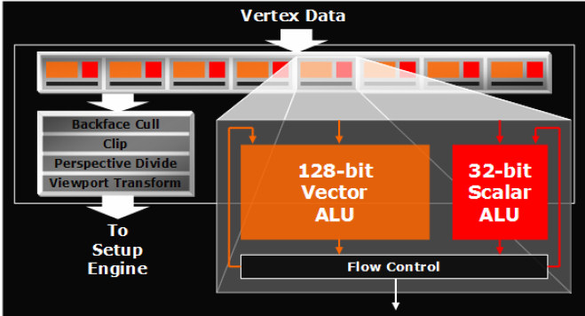
Vertex Shader ALU (ATI Radeon X1900)

It gets the values from input and parameter registers and writes the results to output registers with or without using temporary and address registers as shown on the next figure:

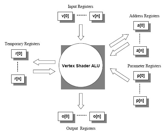
Each of these registers can store four floating point numbers, for instance every input registers from V[0] to V[n] (this means that there are registers with number 0, 1, 2, …, n altogether: n+1 piece of them) can store four 32 bit-long floating point number. Input and parameter registers are read-only, output registers are write-only while address and temporary registers are both readable and writable by the ALU. Input registers store data about vertices. Parameter registers contain values which are valid for more calculations (shader constants), for example the world-view-projection matrix, light positions or light directions. Indexed relative addressing can be performed using the address registers. The shader works on one instruction but on more data parallel at a time, and generally can operate on whole matrices or quaternions. This data format is very useful because most of the transformation and lighting calculations require these kinds of data (vectors and matrices). The fact, that GPUs are designed to operate on more data in one clock cycle parallel enables them to calculate these special tasks much faster than the CPUs of the computers. The most important operations will be described in the next paragraph. Finally the results will be stored in the write-only output registers and passed on to the next stages of the fixed pipeline.

In DirectX 8, the pipeline was programmed with a combination of assembly instructions, High Level Shading Language (HLSL) instructions and fixed-function statements. With the latest APIs it is possible to use only HLSL; in fact, assembly is no longer used to generate shader code with Direct3D 10, but I introduce the assembly operations first. Vertex shader version 1.1 limits the number of instructions to 128 (later versions increase this number dramatically). Operations are in format:

OperationCode DestinationRegister , SourceRegister1 [, SourceRegister2 ] [, SourceRegister3]

Namely, first, the code of the operation comes followed by the name of the destination registers, and finally, the source registers, separated by commas. For example, the following operation adds the values stored in constant register c0 and input register v0 and writes the result into temporary register r0:

add r0, c0, v0

The most important instructions are shown in the next table (vertex shader V1.1):

Name	Description	Instruction slots
add - vs	Add two vectors	1
dp3 - vs	Three-component dot product	1
dst - vs	Calculate the distance vector	1
exp - vs	Full precision 2x	10
log - vs	Full precision log2(x)	10
m3x3 - vs	3x3 multiply	3
m4x4 - vs	4x4 multiply	4
mad - vs	Multiply and add	1
max - vs	Maximum	1
min - vs	Minimum	1
mov - vs	Move	1
mul - vs	Multiply	1
sge - vs	Greater than or equal compare	1
slt - vs	Less than compare	1
sub - vs	Subtract	1

These instructions are enough to make the most of the calculations but there were some which were complicated to perform, for example trigonometric functions needed to be approximated by different Taylor series. Later vertex shader versions made the job of the programmers more comfortable by supporting directly the computing sine and cosine, introducing flow control and new arithmetical instructions. For more details check the MSDN Library.

The output of the vertex shader is a set of vertices, which is passed to the next stages of the graphical pipeline. After interpolation, face culling, viewport mapping, homogeneous division etc. the vertices will arrive to the pixel shader stage.

For more details about vertex shaders, see [7], [6] or [8].

The pixel shader (fragment shader)

Incoming vertices determine the general placement of the objects in the virtual world, but in the end every pixel need to be rendered on the output. The pixel shader makes it possible to order a color to every pixel of the image through the programmer defined instructions. Some of the possible effects are:

Per-pixel lighting
Advanced bump mapping
Volumetric rendering
Procedural textures
Per-pixel Fresnel term
Special shading effects
Anisotropic lighting

The pixel shader operates on pixels before the final stages of the graphic pipeline (alpha, depth and stencil test). Logically, the output of the pixel shader is the corresponding color and depth value for each pixel, interpolated from the input vertices. Using pixel shader bypasses the following parts of the fixed-function pipeline:

Texture access
Texture applications
Blending
Fog application

The working method of the pixel shader's ALU is similar to the vertex shader's. Using the data in the input and parameter registers the result will be calculated with or without the help of the temporary registers and texture samplers. It is finally written into the output register as shown on the next figure:

As you see, the main difference between pixel and vertex shader is the possibility to use texture operations in the pixel shader. Defining a texture as a render-target enables the opportunity to reuse any pre-rendered picture or texture for later calculations alsol. There are some other differences as well, for example, the order of the different kind of instructions is limited and there are several modifiers and masks to slightly change the input or output reading methods in the pixel shader. For more details see the MSDN library.
Similarly to the vertex shader, the pixel shader supports a programming language to define the shader program. But the difference among instruction set versions is significant. The version 1.1-1.3 had a more complex instruction set, but only the reduced instruction set of the version 1.4 will be discussed here (later versions are with version 1.4 backward compatible). Most of the vertex shader instructions became available in the later pixel shader instruction sets, they are today very similar. The most important operations of pixel shader version 1.4 are visible on the next table:

Arithmetic instructions	Description	Instruction slots
add - ps	Add two vectors	1
bem - ps	Apply a fake bump environment-map transform	2
cmp - ps	Compare source to 0	1
cnd - ps	Compare source to 0.5	1
dp3 - ps	Three-component dot product	1
dp4 - ps	Four-component dot product	1
lrp - ps	Linear interpolate	1
mad - ps	Multiply and add	1
mov - ps	Move	1
mul - ps	Multiply	1
nop - ps	No operation	0
sub - ps	Subtract	1

Texture instructions	Description	Instruction slots
texcrd	Copy texture coordinate data as color data	1
texdepth	Calculate depth values	1
texkill	Cancels rendering of pixels based on a comparison	1
texld	Sample a texture	1

High Level Shader Language

High Level Shader Language or HLSL is a programming language for GPUs developed by Microsoft for use with the Microsoft Direct3D API, so it works only on Microsoft platforms and on Xbox. Its syntax, expressions and functions are similar to the ones in the programming language C, and with the introduction of Direct3D 10 API, the graphic pipeline is virtually 100% programmable using only HLSL; in fact, assembly is no longer needed to generate shader code with the latest DirectX versions.

HLSL has several advantages compared to using assembly, programmers do not need to think about hardware details, it is much easier to reuse the code, readability has improved a lot as well, and the compiler optimizes the code. For more details about improvements, see [3].

I have to mention that Cg shader language is equivalent with HLSL language. HLSL and CG are co-developed by Microsoft and nVidia. They have different names for branding purposes. As a part of DirectX API, HLSL compiles only into DirectX code, while Cg compiles into both DirectX and OpenGL code.

HLSL code is used in the demo applications, so I briefly outline here the basics of the language.

Variable declaration

Variable definitions are similar to the ones in C:

float4x4 view_proj_matrix;
float4x4 texture_matrix0;

Here the types are float4x4. This means, 4 x 4 = 12 float numbers are stored in them together, and depending on the operation type, they all participate in the operations. This means, matrix operations can be implemented by them.
Structures

C-like structures can be defined with the keyword struct, as in the following example:

struct MY_STRUCT
{
    float4 Pos : POSITION;
    float3 Pshade : TEXCOORD0;
};

The name of the structure is MY_STRUCT, and it has two fields (the names are Pos and Pshade and the types are float4 and float3). For each field, storing-registers are defined after the colon (:). I discussed the possible register types in the Shader chapter, although the possible register names vary on different Shader versions. The two types in the example are float4 and float3, which means, they are compounded of more float numbers (tree and four floats) which are handled together.
Functions

Functions can be also familiar after using C:

MY_STRUCT main (float4 vPosition : POSITION)

{
    MY_STRUCT Out = (MY_STRUCT) 0;

    // Transform position to clip space
    Out.Pos = mul (view_proj_matrix, vPosition);

    // Transform Pshade
    Out.Pshade = mul (texture_matrix0, vPosition);

    return Out;
}

The name of the function is main, and its returns MY_STRUCT variable. The only input parameter is a float4 variable called vPositions, and it is stored in the POSITION register. Two multiplications are also demonstrated in the example (mul operation), they are performed on different types: a matrix-vector multiplication is shown in the example. By changing only the variables, it is possible to multiply a vector with another vector, or two matrices with each other as well. A list of possible intrinsic functions can be found in Appendix B.
Variable components

It is possible to get the components(x, y, z, w) of the compound variables, as vector and matrix components. It is important to mention, that binary variables are performed also per component:

float4 c = a * b;

Assuming a and b are both of type float4, this is equivalent to:

float4 c;
c.x = a.x * b.x;
c.y = a.y * b.y;
c.z = a.z * b.z;
c.w = a.w * b.w;

Note that this is not a dot product between 4D vectors.

Samplers

Samplers are used to get values from textures. For each different texture-map, which you want to use, a sampler must be declared.

sampler NoiseSampler = sampler_state
{
    Texture = (tVolumeNoise);
    MinFilter = Linear;
    MagFilter = Linear;
    MipFilter = Linear;
    AddressU = Wrap;
    AddressV = Wrap;
    AddressW = Wrap;
    MaxAnisotropy = 16;
};

Effects

The Direct3D library helps developers with an encapsulating technique called effects. Effects are usually stored in a separate text file with .fx or .fxl extension. They can encapsulate rendering states as well as shaders written in ASM or HLSL.

Techniques

An .fx or .fxl file can contain multiple versions of an effect which are called techniques. For example, it is possible to support various hardware versions by using more techniques in a single effect file. A technique can include multiple passes, and it is defined in each pass, which functions are the pixel shader and vertex shader functions:

technique my_technique
{
    pass P0
    {
        VertexShader = compile vs_2_0 vertexFunction();
        PixelShader = compile ps_2_0 pixelFunction();
    }
}

Conclusion

The main ideas were shortly introduced about HLSL in the previous paragraphs. Shader programs of the demo applications are written using HLSL. For more detailed information, see the corresponding chapter or one of the mentioned references ([2] or [3]). A useful HLSL tutorial can be found here: [4]. For a general comparison of shader version 2.0 and 3.0, see [6].

Appendix A

The different DirectX versions and supported shader versions are shown in the following table:

DirectX Version	Pixel Shader	Vertex Shader
8.0	1.0, 1.1	1.0, 1.1
8.1	1.2, 1.3, 1.4	1.0, 1.1
9.0	2.0	2.0
9.0a	2_A, 2_B	2.x
9.0c	3.0	3.0
10.0	4.0	4.0
10.1	4.1	4.1

Pixel shader comparison B

	PS_2_0	PS_2_a	PS_2_b	PS_3_0	PS_4_0
Dependent texture limit	4	No Limit	4	No Limit	No Limit
Texture instruction limit	32	Unlimited	Unlimited	Unlimited	Unlimited
Position register	No	No	No	Yes	Yes
Instruction slots	32 + 64	512	512	≥ 512	≥ 65536
Executed instructions	32 + 64	512	512	65536	Unlimited
Texture indirections	4	No limit	4	No Limit	No Limit
Interpolated registers	2 + 8	2 + 8	2 + 8	10	32
Instruction predication	No	Yes	No	Yes	No
Index input registers	No	No	No	Yes	Yes
Temp registers	12	22	32	32	4096
Constant registers	32	32	32	224	16x4096
Arbitrary swizzling	No	Yes	No	Yes	Yes
Gradient instructions	No	Yes	No	Yes	Yes
Loop count register	No	No	No	Yes	Yes
Face register (2-sided lighting)	No	No	No	Yes	Yes
Dynamic flow control	No	No	No	24	Yes
Bitwise Operators	No	No	No	No	Yes
Native Integers	No	No	No	No	Yes

PS_2_0 = DirectX 9.0 original Shader Model 2 specification.
PS_2_a = NVIDIA GeForce FX-optimized model.
PS_2_b = ATI Radeon X700, X800, X850 shader model, DirectX 9.0b.
PS_3_0 = Shader Model 3.
PS_4_0 = Shader Model 4.
"32 + 64" for Executed Instructions means "32 texture instructions and 64 arithmetic instructions."
Vertex shader comparison

	VS_2_0	VS_2_a	VS_3_0	VS_4_0
# of instruction slots	256	256	≥ 512	4096
Max # of instructions executed	65536	65536	65536	65536
Instruction Predication	No	Yes	Yes	Yes
Temp Registers	12	13	32	4096
# constant registers	≥ 256	≥ 256	≥ 256	16x4096
Static Flow Control	Yes	Yes	Yes	Yes
Dynamic Flow Control	No	Yes	Yes	Yes
Dynamic Flow Control Depth	No	24	24	Yes
Vertex Texture Fetch	No	No	Yes	Yes
# of texture samplers	N/A	N/A	4	128
Geometry instancing support	No	No	Yes	Yes
Bitwise Operators	No	No	No	Yes
Native Integers	No	No	No	Yes

VS_2_0 = DirectX 9.0 original Shader Model 2 specification.
VS_2_a = NVIDIA GeForce FX-optimized model.
VS_3_0 = Shader Model 3.
VS_4_0 = Shader Model 4.

The source of the comparison tables is Wikipedia.
Intrinsic Functions (DirectX HLSL) (Source: MSDN)

The following table lists the intrinsic functions available in HLSL. Each function has a brief description, and a link to a reference page that has more detail about the input argument and return type.

Name	Syntax	Description
abs	abs(x)	Absolute value (per component).
acos	acos(x)	Returns the arccosine of each component of x.
all	all(x)	Test if all components of x are nonzero.
any	any(x)	Test if any component of x is nonzero.
asdouble	asdouble(x)	Convert the input type to a double.
asfloat	asfloat(x)	Convert the input type to a float.
asin	asin(x)	Returns the arcsine of each component of x.
asint	asint(x)	Convert the input type to an integer.
asuint	asuint(x)	Convert the input type to an unsigned integer.
atan	atan(x)	Returns the arctangent of x.
atan2	atan2(y, x)	Returns the arctangent of of two values (x,y).
ceil	ceil(x)	Returns the smallest integer which is greater than or equal to x.
clamp	clamp(x, min, max)	Clamps x to the range [min, max].
clip	clip(x)	Discards the current pixel, if any component of x is less than zero.
cos	cos(x)	Returns the cosine of x.
cosh	cosh(x)	Returns the hyperbolic cosine of x.
cross	cross(x, y)	Returns the cross product of two 3D vectors.
D3DCOLORtoUBYTE4	D3DCOLORtoUBYTE4(x)	Swizzles and scales components of the 4D vector x to compensate for the lack of UBYTE4 support in some hardware.
ddx	ddx(x)	Returns the partial derivative of x with respect to the screen-space x-coordinate.
ddy	ddy(x)	Returns the partial derivative of x with respect to the screen-space y-coordinate.
degrees	degrees(x)	Converts x from radians to degrees.
determinant	determinant(m)	Returns the determinant of the square matrix m.
distance	distance(x, y)	Returns the distance between two points.
dot	dot(x, y)	Returns the dot product of two vectors.
exp	exp(x)	Returns the base-e exponent.
exp2	exp2(x)	Base 2 exponent (per component).
faceforward	faceforward(n, i, ng)	Returns -n * sign(•(i, ng)).
floor	floor(x)	Returns the greatest integer which is less than or equal to x.
fmod	fmod(x, y)	Returns the floating point remainder of x/y.
frac	frac(x)	Returns the fractional part of x.
frexp	frexp(x, exp)	Returns the mantissa and exponent of x.
fwidth	fwidth(x)	Returns abs(ddx(x)) + abs(ddy(x))
GetRenderTargetSampleCount	GetRenderTargetSampleCount()	Returns the number of render-target samples.
GetRenderTargetSamplePosition	GetRenderTargetSamplePosition(x)	Returns a sample position (x,y) for a given sample index.
isfinite	isfinite(x)	Returns true if x is finite, false otherwise.
isinf	isinf(x)	Returns true if x is +INF or -INF, false otherwise.
isnan	isnan(x)	Returns true if x is NAN or QNAN, false otherwise.
ldexp	ldexp(x, exp)	Returns x * 2exp
length	length(v)	Returns the length of the vector v.
lerp	lerp(x, y, s)	Returns x + s(y - x).
lit	lit(n • l, n • h, m)	Returns a lighting vector (ambient, diffuse, specular, 1)
log	log(x)	Returns the base-e logarithm of x.
log10	log10(x)	Returns the base-10 logarithm of x.
log2	log2(x)	Returns the base-2 logarithm of x.
max	max(x, y)	Selects the greater of x and y.
min	min(x, y)	Selects the lesser of x and y.
modf	modf(x, out ip)	Splits the value x into fractional and integer parts.
mul	mul(x, y)	Performs matrix multiplication using x and y.
noise	noise(x)	Generates a random value using the Perlin-noise algorithm.
normalize	normalize(x)	Returns a normalized vector.
pow	pow(x, y)	Returns xy.
radians	radians(x)	Converts x from degrees to radians.
reflect	reflect(i, n)	Returns a reflection vector.
refract	refract(i, n, R)	Returns the refraction vector.
round	round(x)	Rounds x to the nearest integer
rsqrt	rsqrt(x)	Returns 1 / sqrt(x)
saturate	saturate(x)	Clamps x to the range [0, 1]
sign	sign(x)	Computes the sign of x.
sin	sin(x)	Returns the sine of x
sincos	sincos(x, out s, out c)	Returns the sine and cosine of x.
sinh	sinh(x)	Returns the hyperbolic sine of x
smoothstep	smoothstep(min, max, x)	Returns a smooth Hermite interpolation between 0 and 1.
sqrt	sqrt(x)	Square root (per component)
step	step(a, x)	Returns (x >= a) ? 1 : 0
tan	tan(x)	Returns the tangent of x
tanh	tanh(x)	Returns the hyperbolic tangent of x
tex1D	tex1D(s, t)	1D texture lookup.
tex1Dbias	tex1Dbias(s, t)	1D texture lookup with bias.
tex1Dgrad	tex1Dgrad(s, t, ddx, ddy)	1D texture lookup with a gradient.
tex1Dlod	tex1Dlod(s, t)	1D texture lookup with LOD.
tex1Dproj	tex1Dproj(s, t)	1D texture lookup with projective divide.
tex2D	tex2D(s, t)	2D texture lookup.
tex2Dbias	tex2Dbias(s, t)	2D texture lookup with bias.
tex2Dgrad	tex2Dgrad(s, t, ddx, ddy)	2D texture lookup with a gradient.
tex2Dlod	tex2Dlod(s, t)	2D texture lookup with LOD.
tex2Dproj	tex2Dproj(s, t)	2D texture lookup with projective divide.
tex3D	tex3D(s, t)	3D texture lookup.
tex3Dbias	tex3Dbias(s, t)	3D texture lookup with bias.
tex3Dgrad	tex3Dgrad(s, t, ddx, ddy)	3D texture lookup with a gradient.
tex3Dlod	tex3Dlod(s, t)	3D texture lookup with LOD.
tex3Dproj	tex3Dproj(s, t)	3D texture lookup with projective divide.
texCUBE	texCUBE(s, t)	Cube texture lookup.
texCUBEbias	texCUBEbias(s, t)	Cube texture lookup with bias.
texCUBEgrad	texCUBEgrad(s, t, ddx, ddy)	Cube texture lookup with a gradient.
texCUBElod	tex3Dlod(s, t)	Cube texture lookup with LOD.
texCUBEproj	texCUBEproj(s, t)	Cube texture lookup with projective divide.
transpose	transpose(m)	Returns the transpose of the matrix m.
trunc	trunc(x)	Truncates floating-point value(s) to integer value(s)